PINO Applications

In this work, we examine the applications of physics informed neural operators (PINOs). PINOs have demonstrated excellent ability to reproduce results of various test simulations. Here we stress test PINOs over a wide range of problems including the variations of the wave equation, Burgers equation and the shallow water equations. The source code for this work can be found at this repo. We also provide users with a way to try out our code at Argonne’s Data and Learning Hub for Science.

Model

PINOs are a variation of neural operators that incorporate knowledge of physical laws into their loss functions. PINOs have been shown reproduce the results of operators with remarkable accuracy. They employ the Fourier neural operator (FNO) architecture which applies a fast Fourier transform (FFT) to the data and applies its fully connected layers in Fourier space before performing an inverse FFT back to real space. Moreover, this architecture has been demonstrated the ability to perform ability perform zero-shot super-resolution, predicting on higher resolution data having only seen low resolution data. The figure below illustrates the FNO architecture that we use in this study.

PINOs improve upon the FNO architecture by adding physics information such as partial differential equations (PDEs), initial conditions (ICs), boundary conditions (BCs), and other conservation laws. These are done by adding the violation of these laws into the loss function, the network can learn these laws in addition to the data. Rather than using automatic differentiation, these networks use Fourier derivatives to compute the derivatives for the PDE constraints as automatic differentiation is very memory intensive for this type of architecture. This physics knowledge enables the network to learn operators faster and with less training data.

Results

Wave Equation 1D

The 1D wave equation was the first test for our PINOs. This equation computationally simple PDE that is second order in time and models a variety of different physics phenomena. This equation is given by

\begin{align} u_{tt} \left( x,t \right) + c^2 u_{xx}\left( x,t \right)&=0, \\ \nonumber \
u\left( x, 0 \right) &= u_0\left(x\right), \nonumber \\ \nonumber \
x\in \left[ 0,1 \right),& \ t\in \left[0, 1 \right], \nonumber \end{align}

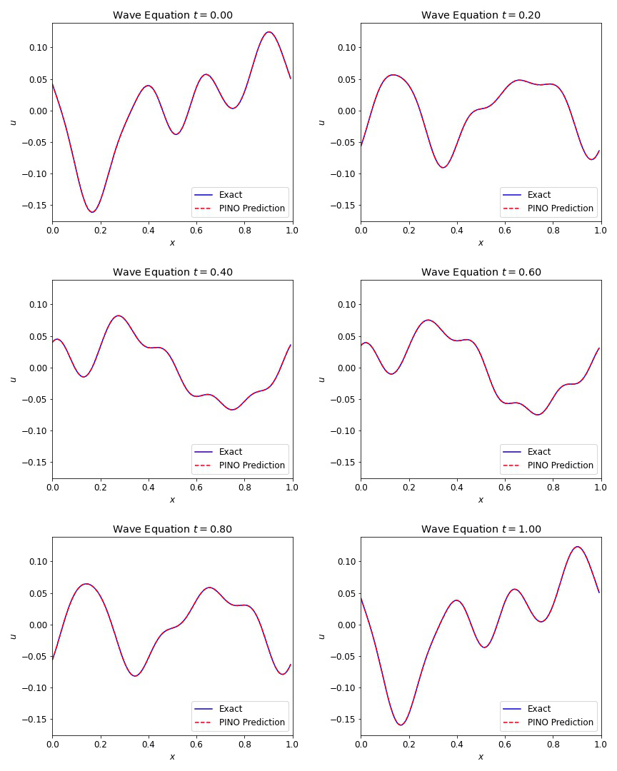
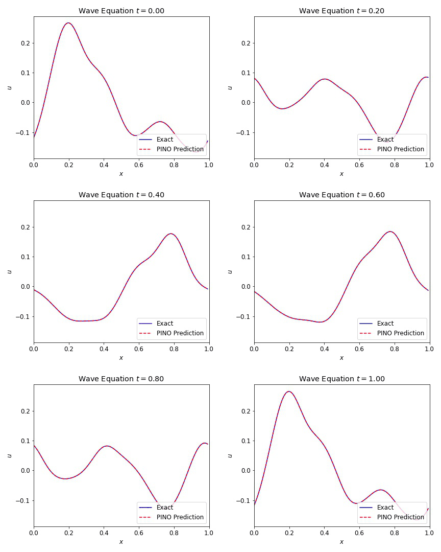
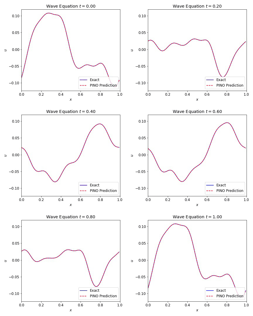
where $c=1$ is our wave speed. We present results below illustrating the ability of the PINO to reconstruct the simulated result for multiple initial conditions. The differences between the simulated data and the PINO are visually indistinguishable.

Wave Equation 2D

We then extended the wave equation into 2D to assess the performance into 2D. This allow us to explore the requirements for adding the additional spatial dimension. In 2D, the wave equation becomes

\begin{align} \label{eq:wave2d} u_{tt} \left( x,y,t \right) + c^2 \left[ u_{xx}\left( x,y,t \right) + u_{yy}\left(x,y,t \right) \right] &=0, \\ \nonumber \
u\left( x,y, 0 \right) &= u_0\left(x,y\right), \nonumber \\ \nonumber \
x,y\in \left[ 0,1 \right),& \ t\in \left[0, 1 \right], \nonumber \end{align}

where $c=1$ is the speed of the wave.

We present result below demonstrating the PINO reconstructing results for the wave equation in 2D and comparing it to the simulated data as well as the error.

Burgers Equation 1D

The 1D Burgers equation serves as a nonlinear test case with for a variety of numerical methods. This allowed us to verify that our PINOs can learn and reconstruct nonlinear phenomena. The equation is given in conservative form by

\begin{align} \label{eq:burgers1d} u_{t}(x, t)+\partial_{x}\left[u^{2}(x, t) / 2\right] &=\nu u_{xx}(x, t), \\ \nonumber \
u(x, 0) &=u_{0}(x), \nonumber \\ \nonumber \
x \in[0,1), & \ t \in[0,1], \nonumber \end{align}

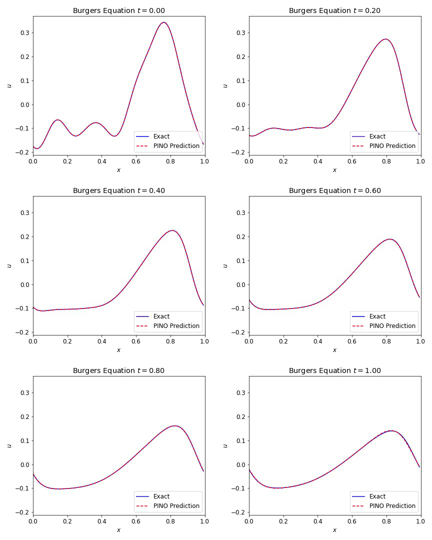
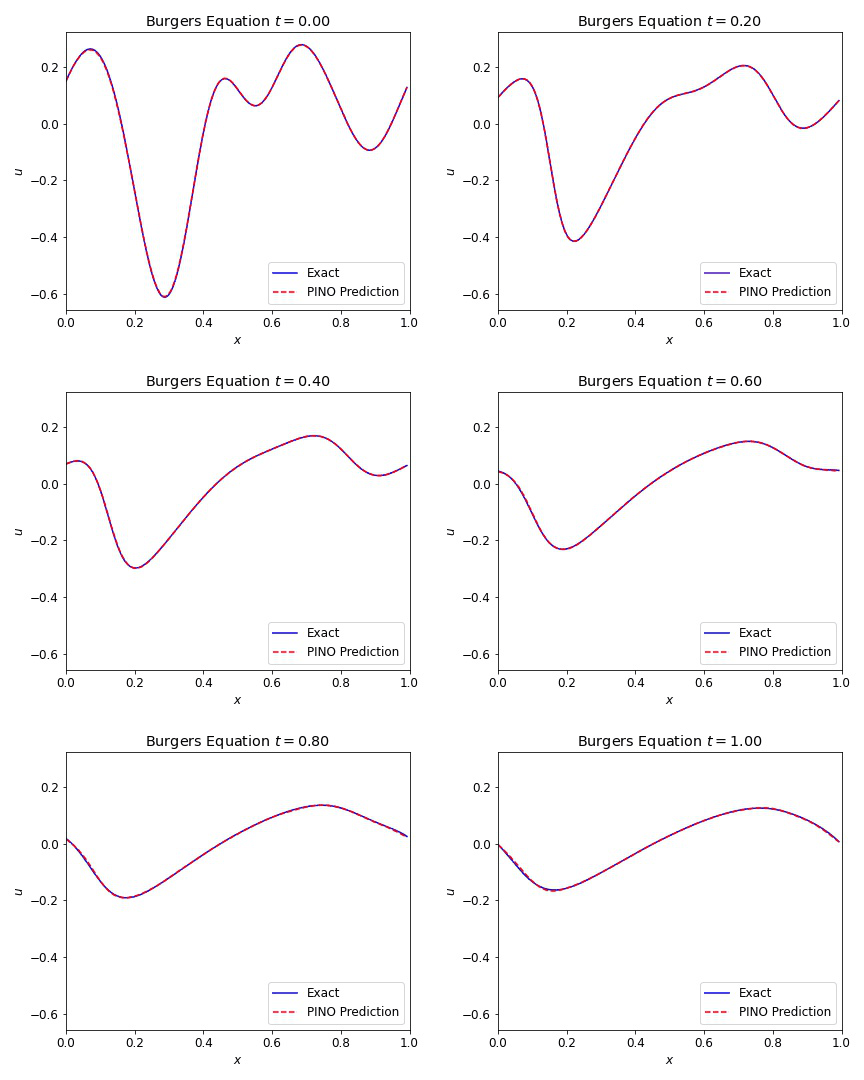
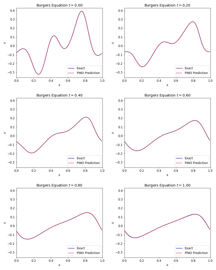
where the viscosity $\nu=0.01$. In the plots below, we illustrate the excellent agreement between the PINO predictions and the simulated values of Burgers equation. As with the wave equation, the PINO results for the 1D Burgers equation are visually indistinguishable from the simulated data.

Burgers Equation 2D Scalar

To verify our model can handle nonlinear phenomena in 2D, we extend the Burgers equation into 2D by assuming the field $u$ is a scalar. The equations take the form

\begin{align} \label{eq:burgers2d} u_{t}(x, y, t)+\partial_{x}\left[u^{2}(x, y, t) / 2\right] + \partial_{y}\left[u^{2}(x, y, t) / 2\right] &=\nu \left[u_{xx}(x, y, t) +u_{yy}(x, y, t)\right], \\ \nonumber \
u(x, y, 0) &=u_{0}(x, y), \nonumber \\ \nonumber \
x,y \in[0,1), & \ t \in[0,1], \nonumber \end{align}

where the viscosity $\nu=0.01$. The plots below the compare the PINO’s predictions to the simulation data with very little error.

Burgers Equation 2D Inviscid

We also looked at cases involving the inviscid Burgers equation in 2D in which we set the viscosity $\nu=0$. This setup is known to produce shocks that can result in numerical instabilities if not handled correctly. We used a finite volume method (FVM) to generate this data to ensure stability in the presence of shocks. In turn, this allowed us to investigate the network’s performance when processing shocks. The equation is given by

\begin{align} \label{eq:burgers2d_inviscid} u_{t}(x, y, t)+\partial_{x}\left[u^{2}(x, y, t) / 2\right] + \partial_{y}\left[u^{2}(x, y, t) / 2\right] &=0, \\ \nonumber \
\quad u(x, y, 0) &=u_{0}(x, y), \nonumber \\ \nonumber \
x,y \in[0,1), \ t \in[0,1]. \nonumber \end{align}

We observe in the plots below that the PINO as able to broadly reconstruct the data in the presence of the shock. Admittedly, the network has dificulty determing the precise location of the shock.

Burgers Equation 2D Vector

Exploring the vectorized form of the 2D Burgers equation allowed us to test how well the model handles coupled fields. Here, we parametrize the system with the fields $u$ and $v$. The equations take the form

\begin{align} \label{eq:burgers2d_vec_I} u_{t}(x, y, t)+u(x, y ,t)u_{x}(x, y, t) + v(x, y, t)u_{y}(x, y, t) &=\nu \left[u_{xx}(x, y, t) +u_{yy}(x, y, t) \right], \\ \nonumber \
\label{eq:burgers2d_vec_II} v_{t}(x, y, t)+u(x, y ,t)v_{x}(x, y, t) + v(x, y, t)v_{y}(x, y, t) &=\nu \left[v_{xx}(x, y, t) +v_{yy}(x, y, t) \right], \\ \nonumber \
u(x, y, 0) =u_{0}(x, y),\ v(x, y, 0) = v_{0}(x, y), \nonumber \\ \nonumber \
x,y \in[0,1), & \ t \in[0,1] \nonumber \end{align}

where the viscosity $\nu=0.01$. We compare the PINO’s results in the figures below to the simulated data and the error. These plots depict the PINO’s ability to accurately handle 2D nonlinear coupled fields.

Nonlinear Shallow Water Equations 2D

To examine the properties of PINOs with 3 coupled nonlinear equations, we examined the ability of the networks to reproduce the nonlinear shallow water equations. These equations are applicable in a number of physical scenerios including tsunami modeling. We assumed that the total fluid column height $\eta(x,y,t)$ was composed of a mean height plus some perturbation, but the initial velicity fields $u(x,y,t)$ and $v(x,y,t)$ were initially zero. These equations are given by

\begin{align} \label{eq:swe_nonlin_I} \frac{\partial(\eta)}{\partial t}+\frac{\partial(\eta u)}{\partial x}+\frac{\partial(\eta v)}{\partial y}&=0, \\ \nonumber \
\label{eq:swe_nonlin_II} \frac{\partial(\eta u)}{\partial t}+\frac{\partial}{\partial x}\left(\eta u^{2}+\frac{1}{2} g \eta^{2}\right)+\frac{\partial(\eta u v)}{\partial y}&=\nu\left(u_{xx} + u_{yy}\right), \\ \nonumber \
\label{eq:swe_nonlin_III} \frac{\partial(\eta v)}{\partial t}+\frac{\partial(\eta u v)}{\partial x}+\frac{\partial}{\partial y}\left(\eta v^{2}+\frac{1}{2} g \eta^{2}\right)&=\nu\left(v_{xx} + v_{yy}\right), \\ \nonumber \
\end{align} \begin{align} \textrm{with} \quad \eta(x,y,0) = \eta_{0}(x,y),\ u(x,y,0)=0,\ v(x,y,0)=0,\ \quad x,y \in[0,1), \ t \in[0,1], \nonumber \end{align}

where the gravitational coefficient $g=1$ and the viscosity coefficient $\nu=0.002$ to prevent the formation of shocks. Below we plot how each of these fields evolves in space and time according to the PINO predictions and to the simulated data. We observe that the error in each of these cases is relatively small.